Cálculo manual de la función de autocorrelación

2022-09-28

Para dar un ejemplo del procedimiento para calcular numéricamente las funciones (de autocovarianza y covarianza cruzada), considere un conjunto artificial de datos generado al lanzar una moneda al aire, y fijando

Construir la siguiente serie de tiempo:

Se simulan diez lanzamientos:

In [18]: import numpy as np
           import pandas as pd
           
           
In [8]: ['Cara' 'Cara' 'Sello' 'Cara' 'Sello' 'Sello'  'Sello' 'Cara'  'Sello' 'Cara']
          ['CaraCaraSelloCaraSelloSelloSelloCaraSelloCara']

De acuerdo a los resultados de los lanzamientos se obtienen los siguientes valores para Xt

In [29]: np.random.rand(10).round(0)
            array([0., 1., 1., 1., 1., 1., 1., 0., 1., 0.])

Escribimos los datos de Xt en forma de serie de tiempo. Para eso se usa la función de pandas "series"

In [24]: X = np.array([ -1,1,  1, -1,  1, -1, -1, -1,  1, -1,  1]) # comienza con X0 =-1 y n=10
            index = pd.date_range(start='1/1/2018', periods=11, freq = "D")

In [25]: # se convierte X en una serie de tiempo
            X = pd.Series(X)
            X.index = index

quiero saber el promedio cada dos días de la serie Yt

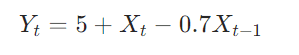
In [26]: Yt = 5 + X - 0.7 * X.shift(1)
            X  = X.iloc[1:]
            Yt = Yt.iloc[1:]
            Yt
            
Out [26]: 2018-01-02    6.7
               2018-01-03    5.3
               2018-01-04    3.3
               2018-01-05    6.7
               2018-01-06    3.3
               2018-01-07    4.7
               2018-01-08    4.7
               2018-01-09    6.7
               2018-01-10    3.3
               2018-01-11    6.7
               Freq: D, dtype: float64            
               
In [27]: Yt.resample("2D").mean()


Out [27]:  2018-01-02    6.0
                2018-01-04    5.0
                2018-01-06    4.0
                2018-01-08    5.7
                2018-01-10    5.0
                Freq: 2D, dtype: float64
                
                
In    [28]: (6.7 + 5.3)/2 ,  (3.3 + 6.7)/2 , (3.3 + 4.7)/2 , (4.7 + 6.7)/2 , (3.3 + 6.7)/2
Out [28]: (6.0, 5.0, 4.0, 5.7, 5.0)

Cálculo de la covarianza de Yt

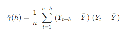
La autocovarianza muestral de la serie Yt se calcula con la siguiente fórmula:

In [29]: Yt - Yt.mean()

Out [29]: 2018-01-02    1.56
               2018-01-03    0.16
               2018-01-04   -1.84
               2018-01-05    1.56
               2018-01-06   -1.84
               2018-01-07   -0.44
               2018-01-08   -0.44
               2018-01-09    1.56
               2018-01-10   -1.84
               2018-01-11    1.56
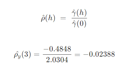
               Freq: D, dtype: float64

Por ejemplo para h=3 la autocovarianza nos da:

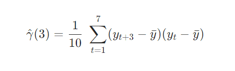
O sea,

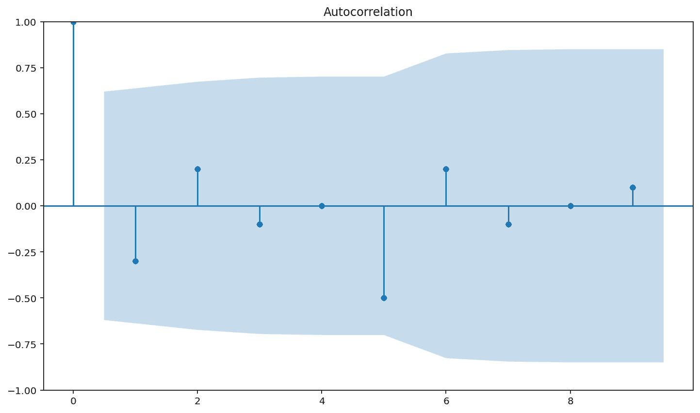
La función de autocorrelación muestral se calcula con la fórmula:

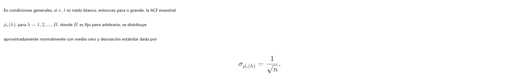
La función de autocorrelación muestral tiene una distribución muestral que permite evaluar si los datos provienen de una serie completamente aleatoria o blanca o si las correlaciones son estadísticamente significativas en algunos rezagos.

In [5]: from pandas.plotting import lag_plot
          from pandas.plotting import autocorrelation_plot
          
In [0]: Y = 5 +  X - 0.7 * X[t-1]

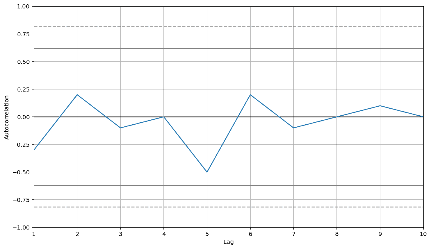
In [36]: autocorrelation_plot(X)

Out [36]: <AxesSubplot:xlabel='Lag', ylabel='Autocorrelation'>

Out [36]

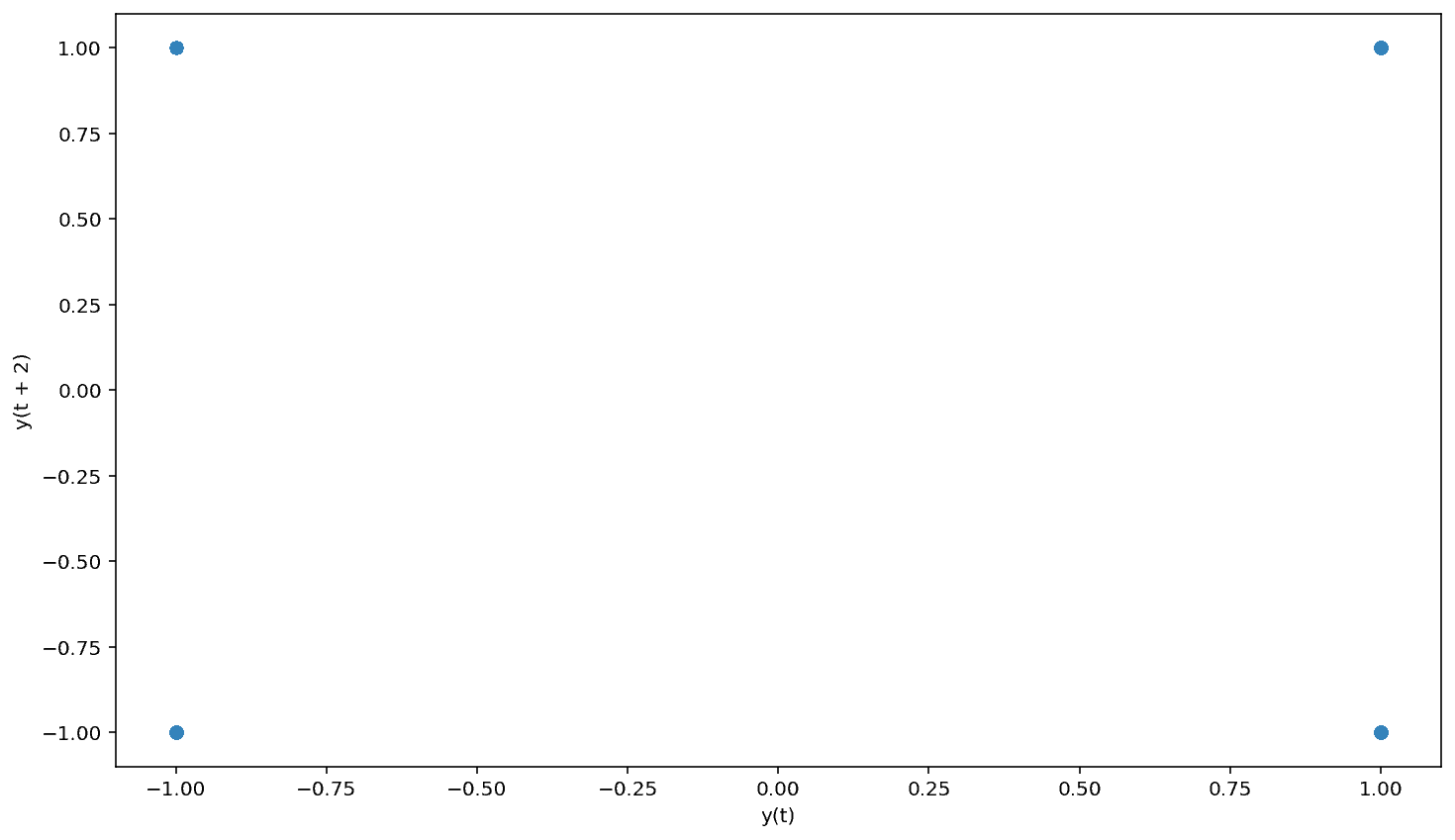
In [39]: lag_plot(X , lag=2)
Out [39]: <AxesSubplot:xlabel='y(t)', ylabel='y(t + 2)'>

Out [39]

In [6]: from statsmodels.graphics.tsaplots import plot_acf
In [8]: plot_acf(X)

Out [8]:

Out [8]